 Casio fx-991MS tips and tricks
Introduction
The Casio fx-991MS is an affordable scientific calculator with many powerful features. Some of these can greatly reduce the effort to solve problems, while others can be abused in interesting and fun ways. Being able to use these features can also be helpful on tests and exams where scientific calculators are allowed but more powerful graphing calculators are not.
On this page, I will show you some advanced and clever tricks that you can do with the calculator. Although the article is for the Casio fx-991MS calculator (and all the tricks mentioned here are guaranteed to work on it), the calculator features and underlying mathematical principles for the tricks are quite general and can be applied to many other calculators as well. (When you understand the trick and your calculator’s features, you’ll be able to translate the instructions for your situation.)
Official Casio manuals
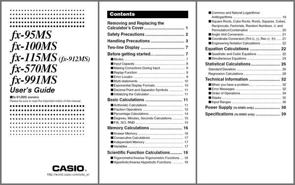
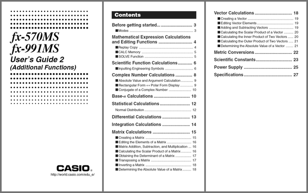
This article assumes that you know the basics of how to use the calculator. If not, please read the user manuals and review how to use the features on the calculator. The official Casio manuals are available as PDF files here:
Contents
-
Standard tricks
- Solve polynomials and linear systems
- Solve arbitrary equations
- Evaluate a function at many points
- Random number generation
- Degree-minute-second conversion
- Numerical differentiation
- Numerical integration
- Display and key test
-
Iterating formulas
-
Simple iterations
- Arithmetic sequence
- Geometric sequence
- Repeated squaring
- Logistic map
- Newton’s method iteration
- Fixed-point iteration
-
Taylor series iterations
- Exponential function
- Cosine function
- Sine function
- Fibonacci sequence iteration
- Greatest common divisor iteration
-
Simple iterations
-
Miscellaneous tricks
- l33tsp34k
- Store 80 numbers
- Wish list
Standard tricks
These tricks are just built-in features of the calculator that are not entirely obvious, because the previous generation of scientific calculators did not have these features.
Solve polynomials and linear systems
To solve a quadratic or cubic polynomial equation:
Go to EQN mode and scroll over to the
Degree?
section (MODE MODE MODE 1 →).Enter the degree (
2or3).Enter the 3 or 4 (real) polynomial coefficients, from highest degree downward.
Scroll up and down through the solution set. Complex-valued solutions are included.
To solve a system of linear equations in 2 or 3 variables:
Go to EQN mode and stay at the
Unknowns?
section (MODE MODE MODE 1)Enter the number of variables, which is also the number of equations (
2or3)Enter the 6 or 12 coefficients of the system of linear equations.
Scroll up and down through the solution vector.
Polynomials equations and linear systems are frequently occurring problems in mathematics and sciences, which makes this calculator feature one of the most useful ones.
Solve arbitrary equations
To solve an arbitrary equation of one variable:
Enter the equation on the formula line. (e.g.,
3X−8=5)Press
SOLVE(SHIFT CALC).Give an initial guess for the variable and press the equals button. Try to give a value near an actual solution, or else solving will be slow or will fail. (However if the equation is linear, then any initial value works.)
Press
SOLVEagain (SHIFT CALC). You may need to wait a few seconds.Read the result. (e.g.,
X=4.333333333)
The calculator uses a form of Newton’s method (as mentioned in the manual) to solve the equation. The algorithm can easily hang, fail, or give a wrong answer, so beware – it is not an automatic solver for all equations.
Tip: Although linear equations are simple to solve in theory, letting the calculator solve it for you can still save you some algebraic manipulation. Here’s an example problem: The 3 angles in a triangle are A, B, and C. B is twice of A. C is triple of B. Find the value of B.
The solution can be found by solving the equation B÷2+B+3B=180.
Evaluate a function at many points
You can evaluate an arbitrary function (of one or more variables) at different arguments without re-entering the function’s definition repeatedly. Procedure:
Enter the expression defining the function. (e.g.
X2+Y)Press
CALC.For each variable in the expression, give it a value.
Read the value of the evaluated expression.
To evaluate the function at another argument, go to step 2 (not step 1).
For example, this makes it much easier to use the rational root theorem to factor or solve polynomials.
Random number generation
The pseudo-variable Ran# (SHIFT .) gives a uniformly distributed random number in the range [0, 1) with a step size of 0.001. It takes on a random value for each instance in a formula and for each evaluation of a formula. (e.g. Ran#+Ran# has a different distribution than 2Ran#.)
To get an integer in the range [0, N), evaluate N×Ran# and mentally discard the fractional part of the result. This can be useful when answering multiple-choice questions, e.g. Go left or right?
.
To get a finer step size, use Ran#+0.001Ran# (step size 10−6) or Ran#+0.001Ran#+0.000001Ran# (step size 10−9).
Degree-minute-second conversion
We inherited the sexagesimal (base-60) number system from the Babylonians. While it makes some division problems easier for mental arithmetic, generally speaking decimal fractions are far easier to work with in practice. But for those times when you do need to work in sexagesimal or convert between it and decimal, this calculator comes to the rescue. It supports number input in degree-minute-second format, and can convert to and from decimal format. See the manual for details, or just play around with the °′″ button.
Obviously, this feature is useful for doing calculations with angles expressed in DMS notation. But I think it’s less well known that it helps calculations involving time, too. Don’t you remember that there are 60 minutes in an hour and 60 seconds in a minute? These subdivisions are the same as the DMS scheme.
To illustrate how DMS features can be used to solve time-related problems, I present some example exercises:
-
You arrived at work at 08:42:44 and left at 17:24:59. How long were you present at work?
Answer:
17°24°59° − 08°42°44°, which yields8°42°15. This means 8 hours, 42 minutes, and 15 seconds. Pressing the°′″button swiftly converts this answer to about 8.704 hours. -
You start driving at 21:30:00 at a speed of 30 m/s, and you need to travel 150 km. At what time will you reach your destination?
Answer:
21°30° + 150×1000÷30÷3600, which yields 22:53:20 (exact).
Numerical differentiation
The numerical differentiation operation (SHIFT ∫dx) takes 2 or 3 arguments:
- The function of X to differentiate
- The point where the derivative is evaluated at
- The change in X (optional)
For example: d/dx(X^X,0.5) = 0.216976666. (The true value is about 0.216977710.)
Numerical integration
The numerical integration operation (∫dx) takes 3 or 4 arguments:
- The function of X to integrate
- The lower limit
- The upper limit
- The amount of partitioning (optional)
If the amount of partitioning is n, then the number of partitions is 2n. See User’s Guide 2 for more details.
Example of usage, while varying the amount of partitioning:
∫(X−1,1,2,1)= 0.7∫(X−1,1,2,2)= 0.69∫(X−1,1,2,3)= 0.6932∫(X−1,1,2,4)= 0.69315∫(X−1,1,2,5)= 0.693147∫(X−1,1,2,6)= 0.6931472∫(X−1,1,2,7)= 0.69314718∫(X−1,1,2,8)= 0.693147181∫(X−1,1,2,9)= 0.69314718
The true value is ln 2, approximately 0.693147181.
Warning: Most functions integrate much more slowly and yield more error than this example.
Display and key test
To enter the calculator’s display and key test mode, press and hold SHIFT and 7, then ON. To exit the test at any time, press ON. (Note: Pressing 7 is not necessary on some older versions of this calculator.)
The first phase is the display test. Press SHIFT to step through the sequence of LCD patterns:
- All segments on
- All segments off
- Half of segments on
- The other half of segments on
- Many copies of a single digit, from 0 to 9
The last display test shows 999999999999. Pressing SHIFT again starts the second phase, the key test. To complete the test, press every key (except ON) in order from left to right, top to bottom. The number on the screen increments every time you correctly hit the next key in the sequence. Don’t press ON unless you intend to quit!
Iterating formulas
A major difference between this calculator and older scientific calculators is that this calculator does not evaluate the expression while you input it. After you finish entering the expression, you press the equals key (=) and the calculator evaluates the expression all at once.
The most recent expression evaluated can be re-evaluated simply by pressing the equals key. The result of each evaluation is always saved in the answer variable (Ans). For single-statement iterations, it is most convenient to use Ans as the iterated variable. For example, Ans+1 is functionally equivalent but easier to type than X=X+1.
Multi-statement iterations can be written by using colon (ALPHA ∫dx) to separate the statements. When evaluating, press the equals key once per statement, and the calculator evaluates them in sequence. When all the statements in the line have been evaluated, pressing the equals key will go back to evaluating the first statement. For example, A=A+2:B=B−3 is a multi-statement line.
Remember to give initial values to all the variables used in the iterations.
Simple iterations
- Arithmetic sequence
-
For example, starting at 0 and counting up by 1:
Initialize: Evaluate
0(sets Ans to 0).Iterate: Evaluate
Ans+1.
- Geometric sequence
-
For example, starting at 1 and doubling:
Initialize: Evaluate
1(sets Ans to 1).Iterate
2Ans.
- Repeated squaring
-
For example, starting at 1.000000001 and squaring:
Initialize: Evaluate
1.000000001(sets Ans to 1.000000001).Iterate
Ans2.
(The value overflows after 38 iterations.)
- Logistic map
-
For example, the chaos at r = 4:
Initialize: Evaluate
0.2(sets Ans to 0.2).Iterate
4Ans(1−Ans)and watch the randomness.
Newton’s method iteration
To solve an equation of the form f(x) = 0:
Set Ans to an initial value close to a root (solution).
Iterate the expression Ans − f(Ans)/f′(Ans), where f′ is the derivative of f.
For example, to solve x2 − 3 = 0:
Initialize: Evaluate
1000(Ran#−0.5).Iterate
Ans−(Ans2−3)/(2Ans).
After a number of iterations, the result should converge to 1.732050808 or −1.732050808, depending on the initial value.
Fixed-point iteration
It is possible to solve equations of the form f(x) = x by simply iterating xnext = f(x).
Examples:
Iterating
cos Ans, the answer converges to 0.739085133 in radians mode and 0.999847741 in degrees mode.Iterating
e−Ans(i.e., e−Ans), the answer converges to 0.567143290.
Unfortunately, fixed-point iteration is generally slower and less reliable than Newton’s method.
Taylor series iterations
We can manually simulate some elementary functions using naive Taylor series.
- Exponential function
-
Initialize
Xwith the argument of your choice.Initialize:
Y=1,A=0,C=0Iterate:
A=A+Y : Y=YX÷(C+1) : C=C+1Read the answer from A.
- Cosine function
-
Initialize
Xwith the argument of your choice.Initialize:
Y=1,A=0,C=0Iterate:
A=A+Y : Y=−YX2÷(C+1)÷(C+2) : C=C+2Read the answer from A.
- Sine function
-
Initialize
Xwith the argument of your choice.Initialize:
Y=X,A=0,C=1Iterate:
A=A+Y : Y=−YX2÷(C+1)÷(C+2) : C=C+2Read the answer from A.
Fibonacci sequence iteration
Procedure:
Initialize:
A=0,B=1Iterate:
C=A+B : A=B : B=C
Greatest common divisor iteration
This is based on the original Euclidean algorithm, which uses repeated subtraction rather than the modulus (remainder) operation. The procedure:
Set the mode to complex numbers (
MODE 2). (This is needed in order to use the absolute value function.)Initialize: Set A and B to be the natural numbers whose GCD will be computed.
Iterate:
A = A − B (tanh(20A−20B) + Abs tanh(20A−20B)) ÷ 2 : B = B − A (tanh(20B−20A) + Abs tanh(20B−20A)) ÷ 2. (Quite a mouthful, isn’t it?)When A and B converge to the same number, that number is the GCD answer.
Note that the function f(x) = (tanh(20x) − |tanh(20x)|) / 2 hackily emulates a step function, with f(x) = 0 for x ≤ 0 and f(x) = 1 for x ≥ 1. (This is due to the finite precision and rounding.)
Thanks to Bojan Petrovic for suggesting this trick!
Miscellaneous tricks
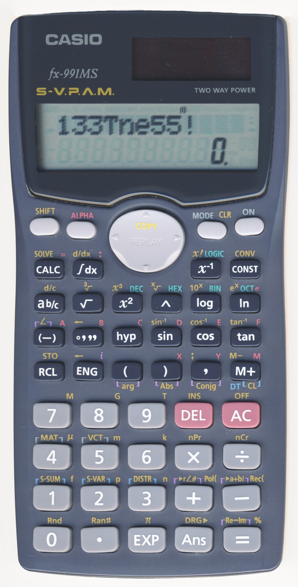
l33tsp34k
The calculator contains a palette of symbols, which can be used to spell out words and phrases in l33tsp34k. The complete (Latin) alphabet cannot be spelled out, but this can make the exercise more fun.
| Letter | Character | Meaning | Key sequence |
|---|---|---|---|
| A | A | Variable A | ALPHA (−) |
4 | Digit 4 | 4 | |
α | Fine structure constant | CONST 10 | |
| B | B | Variable B | ALPHA °′″ |
8 | Digit 8 | 8 | |
| C | C | Variable C | ALPHA hyp |
C | Combination function | SHIFT + | |
| D | D | Variable D | ALPHA sin |
| E | E | Variable E | ALPHA cos |
E | E notation separator | EXP | |
e | Exponential function | SHIFT ln | |
e | Elementary charge | CONST 23 | |
e | Euler’s number | ALPHA ln | |
3 | Digit 3 | 3 | |
| F | F | Variable F | ALPHA tan |
F | Faraday constant | CONST 22 | |
f | SI prefix femto | SHIFT 1 | |
| G | G | SI prefix giga | SHIFT 8 |
G | Gravitational constant | CONST 39 | |
g | Standard gravity | CONST 35 | |
| H | h | Planck constant | CONST 06 |
| I | i | Imaginary unit | ENG (only in complex mode) |
1 | Digit 1 | 1 | |
| K | k | SI prefix kilo | SHIFT 6 |
k | Boltzmann constant | CONST 25 | |
| L | 1 | Digit 1 | 1 |
| M | M | Variable M | ALPHA M+ |
M | SI prefix mega | SHIFT 7 | |
m | SI prefix milli | SHIFT 5 | |
| N | n | SI prefix nano | SHIFT 3 |
| O | 0 | Digit 0 | 0 |
| P | P | Permutation function | SHIFT × |
p | SI prefix pico | SHIFT 2 | |
| R | R | Ideal gas constant | CONST 27 |
| S | 5 | Digit 5 | 5 |
| T | T | SI prefix tera | SHIFT 9 |
t | Celsius temperature | CONST 38 | |
7 | Digit 7 | 7 | |
| U | u | Unified atomic mass unit | CONST 17 |
| X | X | Variable X | ALPHA ) |
× | Times | × | |
| Y | Y | Variable Y | ALPHA , |
| Z | 2 | Digit 2 | 2 |
The letters that cannot be represented are J, Q, V, W. Discovering the punctuation that can be entered is left as an exercise for the reader.
Store 80 numbers
In the SD mode, you can store a sequence of up to 80 numbers, which persist even after a power cycle. To store a number, enter a literal number or an expression, then pressing DT (M+). To retrieve the numbers, scroll through the sequence of stored numbers by pressing up or down (↑, ↓).
In theory, any information can be stored as numbers. (Modern digital computers are built completely on this fact.) For example, if you want to store text on the calculator, just devise a coding scheme that maps between letters and numbers. Note that with the precision available, each number on this calculator can hold up to about 40.7 bits of information.
Wish list
It would be nice if the Casio fx-991MS had these features. They’re not found on other scientific calculators, but they are sometimes found on graphing calculators, and they’re certainly available on general-purpose computers (even smartphones):
Integer division, modulo, power modulo, reciprocal modulo, greatest common divisor
Gamma function (real-valued factorial), other special functions
Fully implemented complex number functions (e.g. sine of complex number, exp of complex number, etc.)